The term ‘categorical data’ is used to describe information that can be divided into distinct groups or categories.
These categories are often labels or names that describe attributes of the data, rather than numerical measurements.
For example, in sport, categorical data might include player positions (e.g., “Forward”, “Defender”) or match outcomes (e.g., “Win”, “Loss”, “Draw”).
Categorical vs. numerical data
Categorical data consists of labels or groups. It doesn’t have inherent numerical meaning (e.g., team names or player roles can’t be said to be ‘more than’ or ‘smaller than’ each other).
In contrast, numerical data consists of numbers that represent measurable quantities (e.g., the number of goals scored, the distance run).
Categorical vs. continuous data
Categorical data divides data into discrete groups with no in-between values (e.g., match outcomes are specifically Win, Loss, or Draw).
In contrast, continuous data represents data that can take any value within a range (e.g., player height or weight).
Categorical vs. ordinal data
Nominal data (one type of categorical data) has categories without a meaningful order (e.g., team names). It can’t be ranked.
Ordinal data (another type of categorical data) has categories with a clear order or ranking (e.g., 1st, 2nd, 3rd in a league).
Note the key distinction: categorical data groups information into qualitative categories, whereas numerical or continuous data provides measurable values that allow for arithmetic operations. Ordinal data can be ordered into ranks, whereas nominal data can’t be ordered in any meaningful way.
Categorical data is very common in sport analytics. We often use it to classify and group information, which in turn makes it easier to identify patterns and trends.
For example, categorical data might include player positions, match outcomes (e.g., win, loss, draw), event types (e.g., fouls, passes, goals), and environmental conditions (e.g., weather, stadium type). These categories often capture qualitative aspects of the game, which can be quantified to (for example) inform strategies or evaluate performance.
In sport, categorical data is both common and very useful.
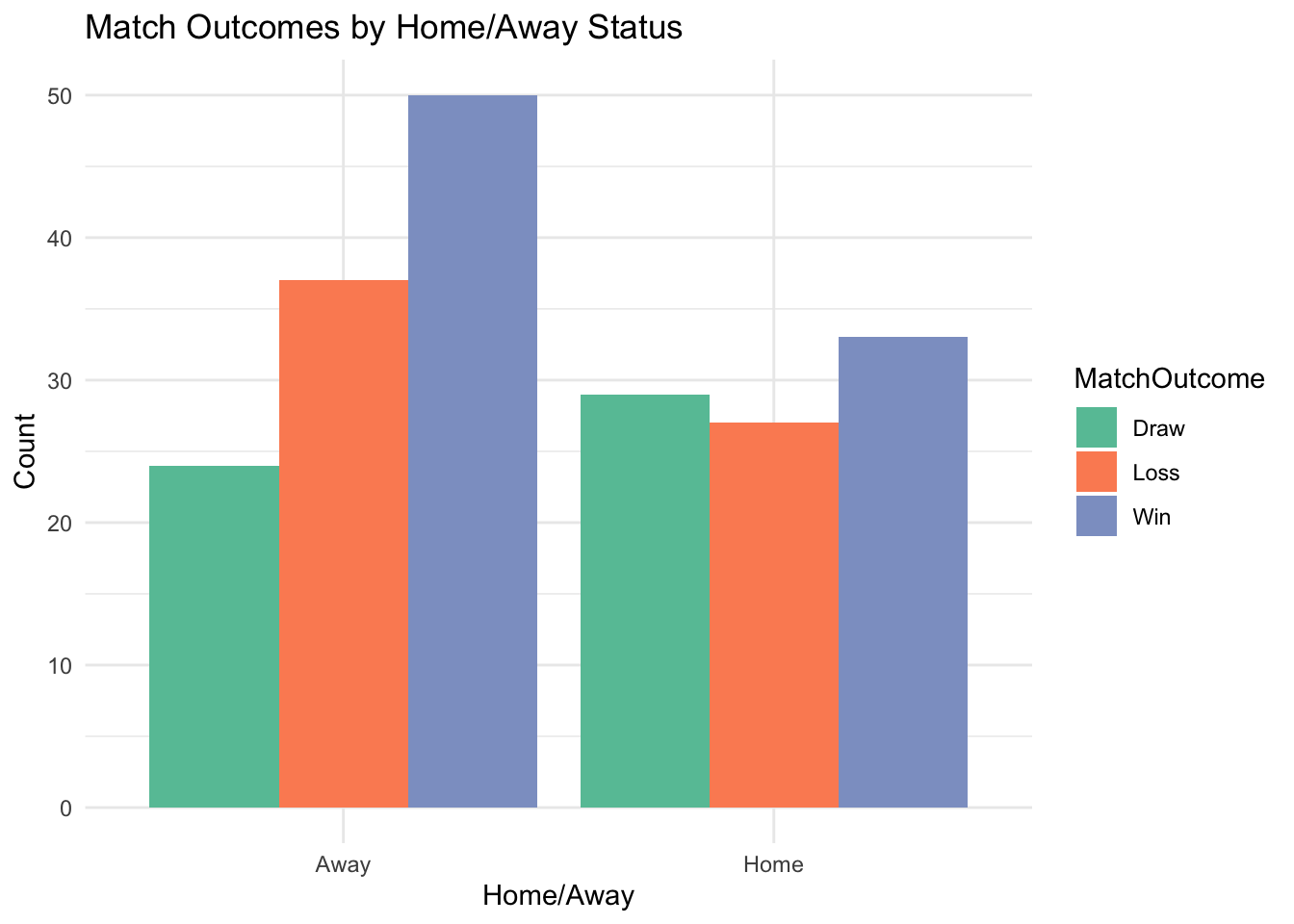
For example, understanding how a team performs in different categories of game situation (e.g., home versus away), or under different weather conditions—can suggest underlying strengths and weaknesses. Similarly, you might want to use categorical data (like player positions) to help model performance metrics, such as the likelihood of a midfielder scoring compared to a forward.
Analysis of categorical data presents some interesting challenges:
It requires encoding to be used in statistical and machine learning models, as most algorithms cannot process non-numeric data directly.
‘Encoding’ categorical data is the process of converting categories into a numeric format that can be used by statistical models or machine learning algorithms. This is covered in more detail below.
Second, as noted above, we need to think about the distinction between nominal and ordinal data.
Nominal categories, such as team names, have no inherent order, whereas ordinal categories, such as performance ratings, do.
Another common issue is high ‘cardinality’, where a categorical variable contains many unique values.
For example, in a dataset of football matches, the “team name” variable might include hundreds of entries, making it difficult to process effectively. Additionally, missing or inconsistent categorical data—such as variations in how categories are labeled—can lead to inaccuracies or biases in models.
Basically, we need to make sure our categorical data are accurately represented and appropriately used in our downstream analysis.
Encoding categorical variables is a critical step in preparing data for analysis. As mentioned above, most statistical models and machine learning algorithms cannot directly handle categorical data, so variables of this type be transformed into a numeric format while still preserving the meaning of the categories.
Common encoding methods include:
One-Hot Encoding: This converts each category into a separate binary variable (e.g., “Forward,” “Defender,” “Midfielder,” and “Goalkeeper” become four separate columns, with a 1 indicating the category for a given row). This method is useful for nominal data but can lead to high-dimensional datasets if there are many categories.
Label Encoding: This assigns a unique integer to each category (e.g., “Forward” = 1, “Defender” = 2). While compact, this method can misrepresent nominal data by implying an ordinal relationship between categories. You’re likely to have encountered this type of encoding before.
Ordinal Encoding: This technique is specifically used for ordered categories (e.g., “Beginner,” = 1, “Intermediate” = 2, “Advanced” = 3), where numeric values represent the rank.
The choice of encoding method depends on the type of categorical variable (nominal or ordinal) and the downstream analysis we’re planning.
For example, one-hot encoding works well with algorithms like logistic regression, while decision trees can often handle label-encoded variables directly.
Missing data is a common issue in categorical variables and requires careful handling to avoid biases or misinterpretations. Techniques we’ve learned previously, like median imputation, obviously don’t work with categorical data!
This is why it’s important to remember that not every numerical value is actually a number. If your data includes label encoding, for example, you might be tempted to calculate the mean or median of the variable, where this doesn’t actually make any sense.
Some approaches to dealing with missing categorical data include:
Mode imputation: Replacing missing values with the most frequent category. This method is simple but can distort the distribution if one category is overly dominant.
Creating “Missing” Categories: We can add a new category to represent missing values. This approach is particularly useful when missingness itself may convey information.
Predictive Imputation: This approach uses machine learning models to predict missing categories based on other features. While more accurate, it is also more complex.
Choosing the right method depends on the context of the data and the importance of the ‘missingness’ to the analysis.
As for other variable types, exploring categorical data helps us identify patterns, relationships, and potential issues.
Common techniques for EDA include:
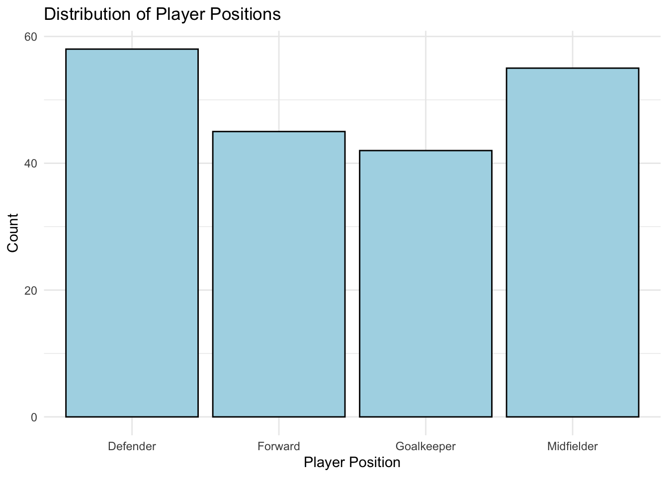
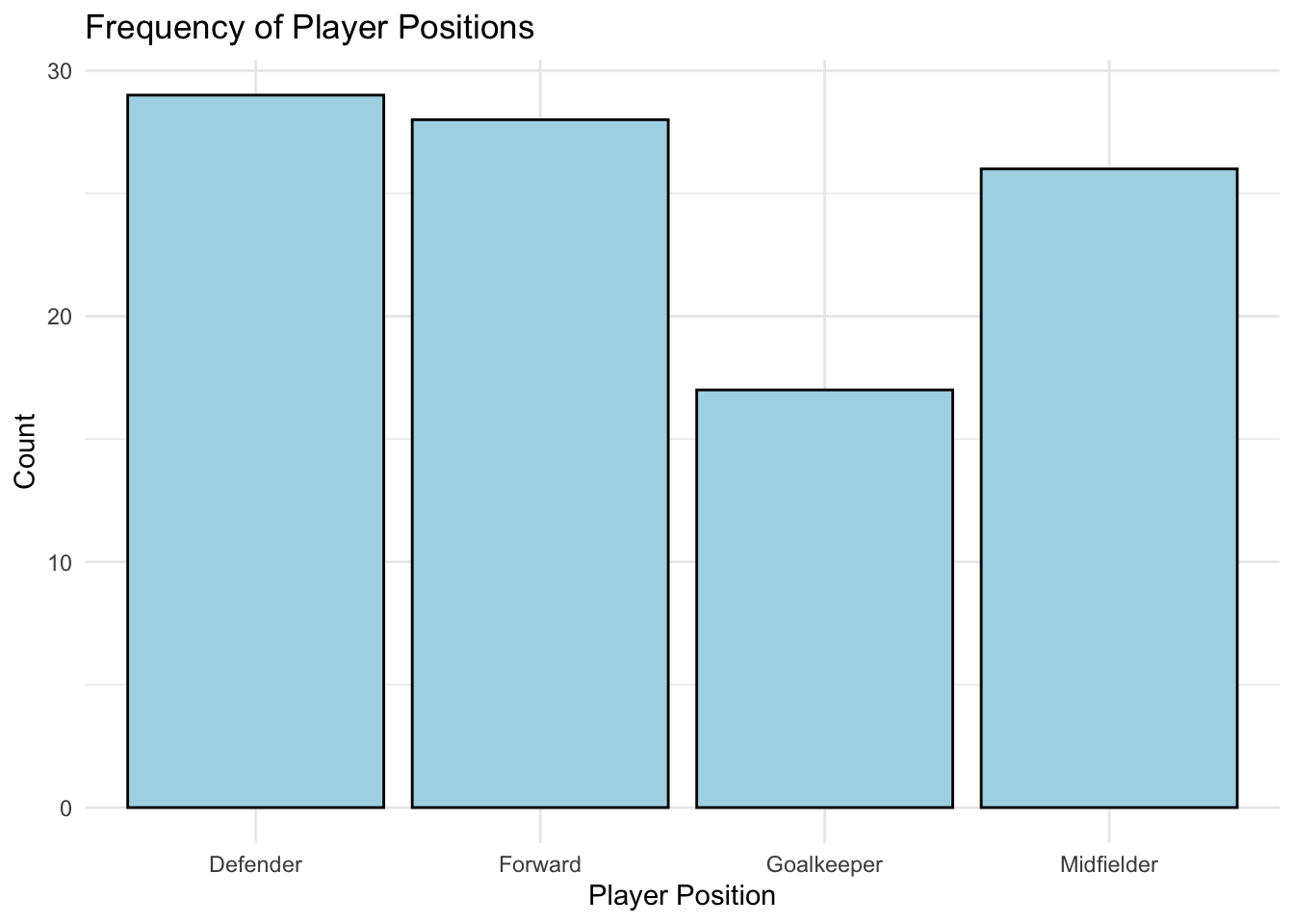
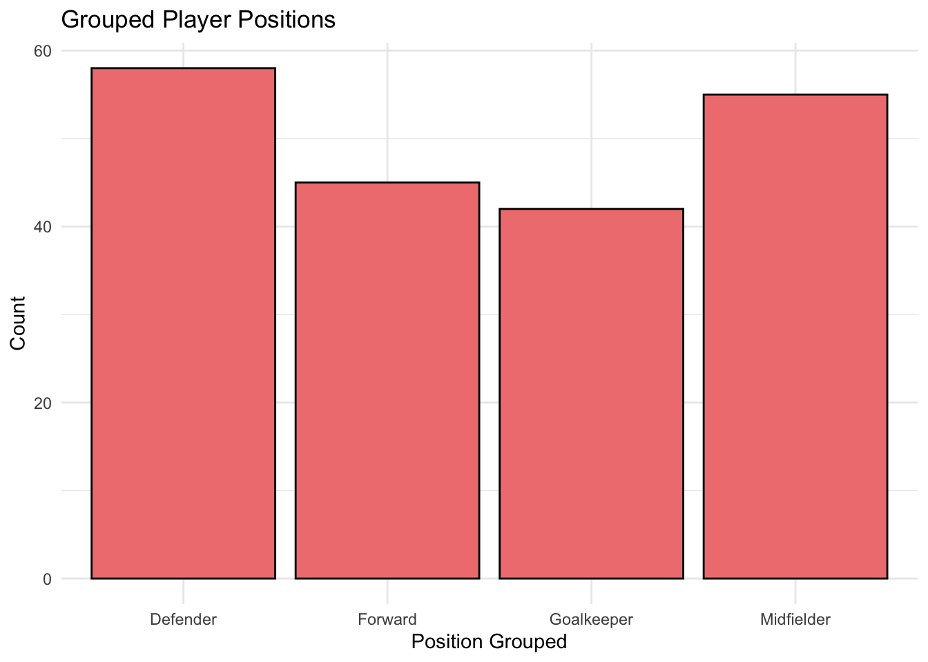
Frequency Distribution: Examining how often each category occurs. For example, analysing player positions might reveal an imbalance in the dataset, such as more forwards than goalkeepers.
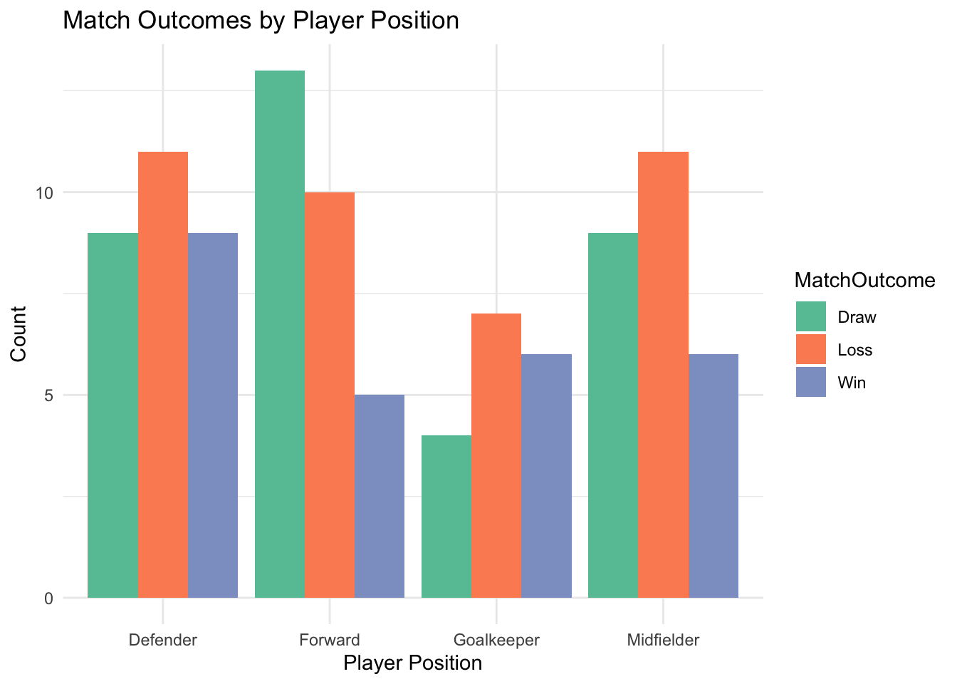
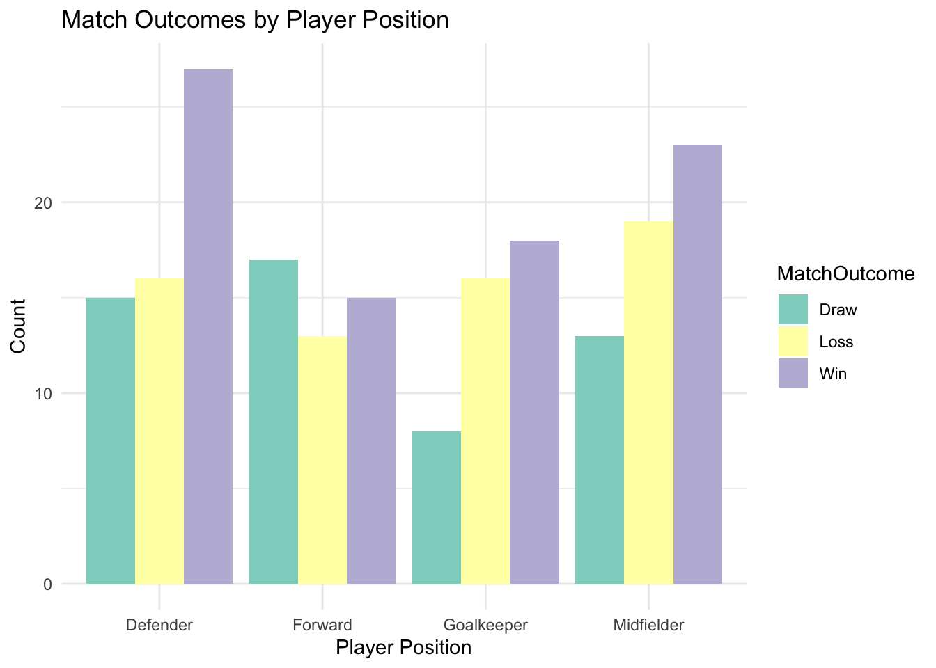
Contingency Tables: Summarising relationships between two categorical variables (e.g., player position vs. match outcome).
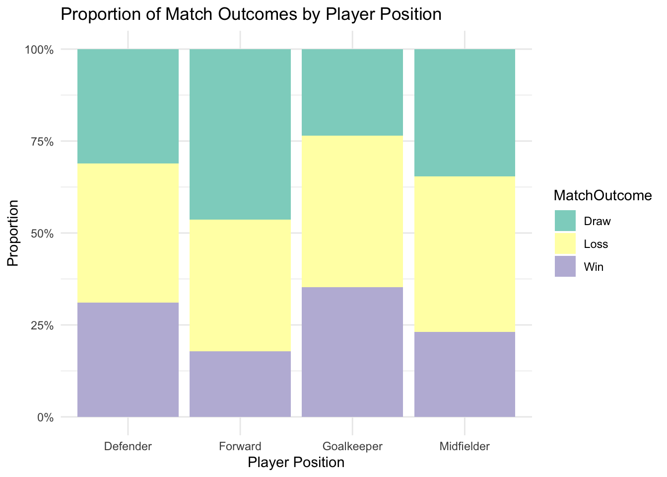
Visualisations: Using bar charts, mosaic plots, and grouped bar charts to reveal distributions and relationships.
These methods provide an essential first step in understanding categorical data, helping inform preprocessing decisions and identify potential challenges like sparsity or imbalance.
Logistic regression is a common method for analysing categorical data, particularly when the outcome variable is binary (e.g., win/loss, goal/no goal).
Unlike linear regression, logistic regression models the probability of an outcome using a logistic function, ensuring that predicted probabilities stay between 0 and 1.
For categorical predictors, encoding plays a key role (see above).
Nominal variables are typically one-hot encoded to create binary dummy variables. Ordinal variables can be directly included if their numerical representation reflects their order.
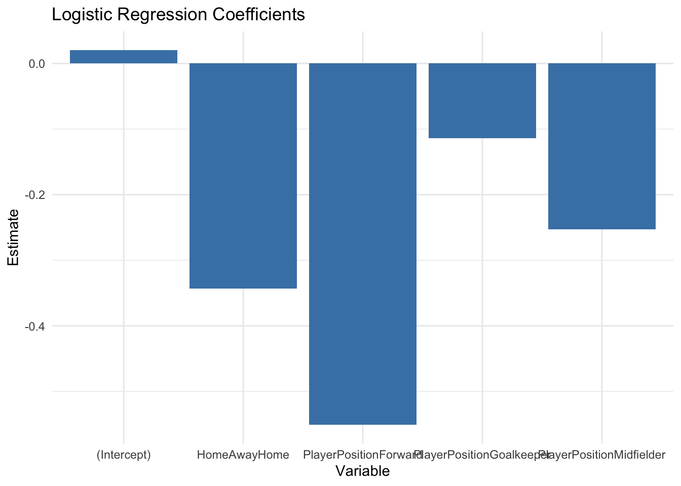
For example, a logistic regression model might predict the probability of a team winning based on factors like the player’s position and home/away status. Coefficients from the model provide insights into the impact of each variable while holding others constant.
The Chi-square test can be used to evaluate whether two categorical variables are independent. It compares the observed frequencies in each category combination with expected frequencies under the assumption of independence.
For example, in a sport dataset, we might test whether player position (Forward, Midfielder, Defender, Goalkeeper) is independent of match outcome (Win, Loss, Draw). A significant result would indicate a relationship between the two variables.
Beyond testing independence, it’s often useful to quantify the strength of relationships between categorical variables (much like we’d use a correlation for continuous data).
We can use:
Cramer’s V, which measures association strength for variables with more than two categories.
Phi Coefficient, which is suitable for 2x2 tables.
These measures give us additional insights into categorical data relationships, aiding in feature selection and interpretation.
Contingency tables summarise the joint distribution of two categorical variables, providing a clear snapshot of their relationship. For instance, a table showing the distribution of player positions by match outcomes can reveal patterns, such as defenders being associated more with draws than forwards.
Proportions within contingency tables allow for deeper exploration. Row or column proportions can highlight trends while controlling for differences in category frequencies.
Call:
glm(formula = WinBinary ~ PlayerPosition + HomeAway, family = "binomial",
    data = sports_data)

Coefficients:
                         Estimate Std. Error z value Pr(>|z|)
(Intercept)              -0.04997    0.49984  -0.100   0.9204
PlayerPositionForward    -0.89170    0.66332  -1.344   0.1789
PlayerPositionGoalkeeper  0.11877    0.67534   0.176   0.8604
PlayerPositionMidfielder -0.59193    0.64372  -0.920   0.3578
HomeAwayHome             -1.23267    0.48656  -2.533   0.0113 *
---
Signif. codes:  0 '***' 0.001 '**' 0.01 '*' 0.05 '.' 0.1 ' ' 1

(Dispersion parameter for binomial family taken to be 1)

    Null deviance: 114.61  on 99  degrees of freedom
Residual deviance: 105.64  on 95  degrees of freedom
AIC: 115.64

Number of Fisher Scoring iterations: 4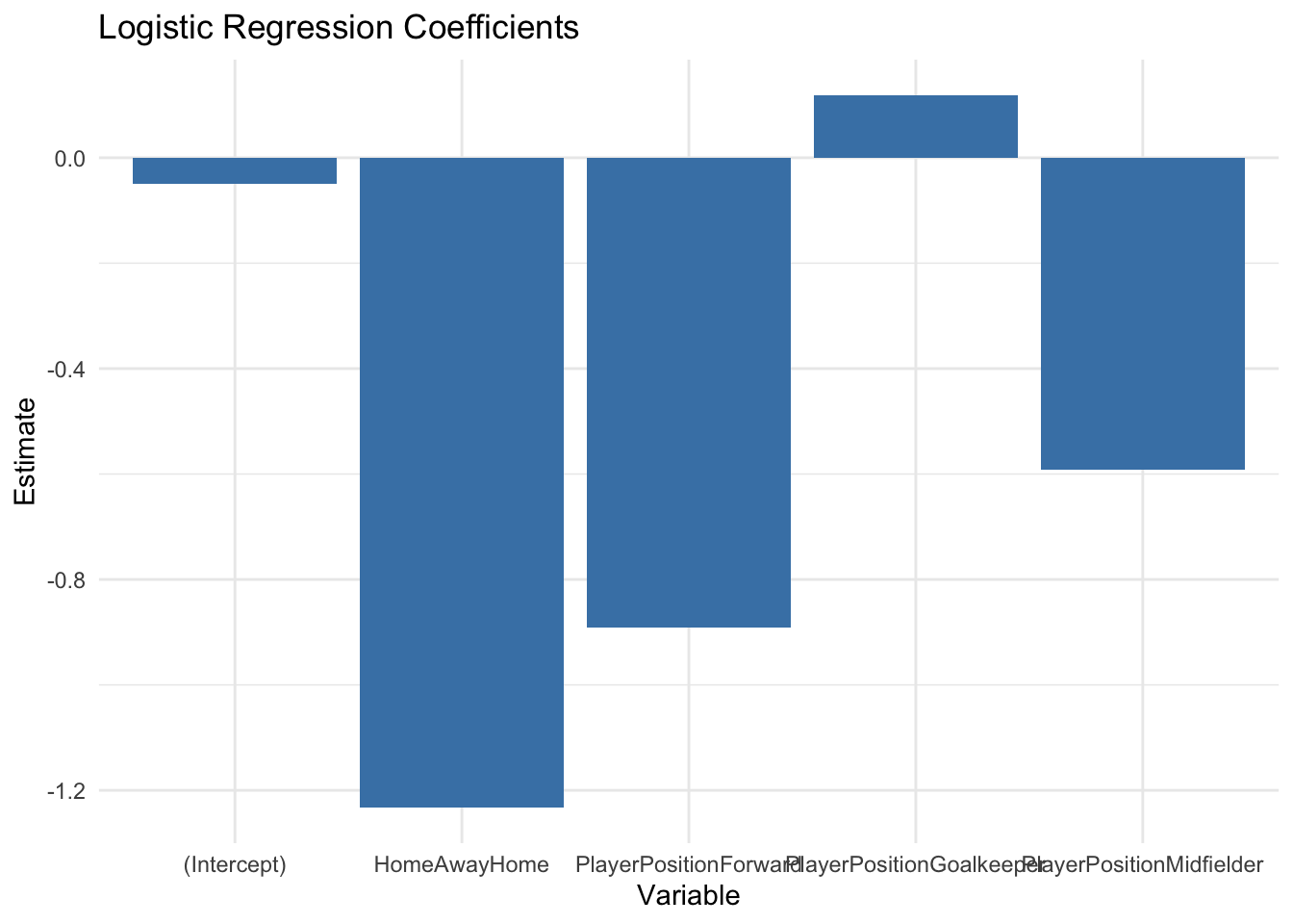
    Pearson's Chi-squared test

data:  contingency_table
X-squared = 3.642, df = 6, p-value = 0.725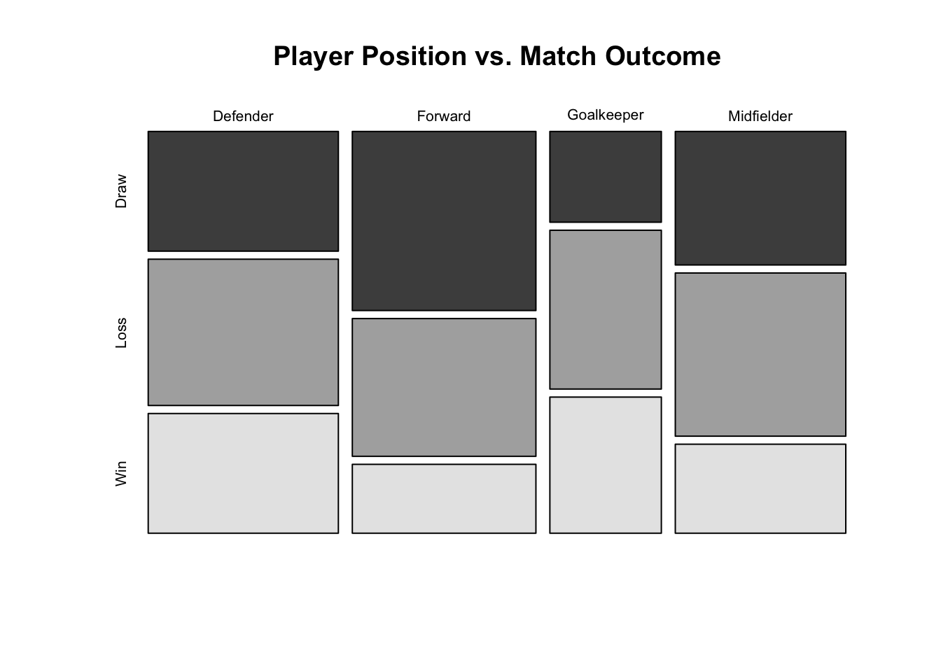
High cardinality occurs when a categorical variable contains many unique categories, such as player names or team IDs.
This creates some challenges for modeling and interpretation, including:
Dimensionality explosion: One-hot encoding can create an excessive number of columns, which may lead to overfitting and slow computation.
Sparse data: Many categories might have very few occurrences, reducing their statistical reliability.
To address high cardinality, we can use a few different techniques including:
Category grouping: Combine less frequent categories into an “Other” group. For instance, we might group less common player positions in a dataset of non-elite players. If your primary focus is on forwards, for example, you might not need to create separate categories for every other position and go with ‘other’ instead.
Feature hashing: We can use a hashing function to map categories to a fixed number of columns, reducing dimensionality while preserving information.
Frequency encoding: We can replace each category with its occurrence count in the dataset, providing numerical representation while retaining granularity.
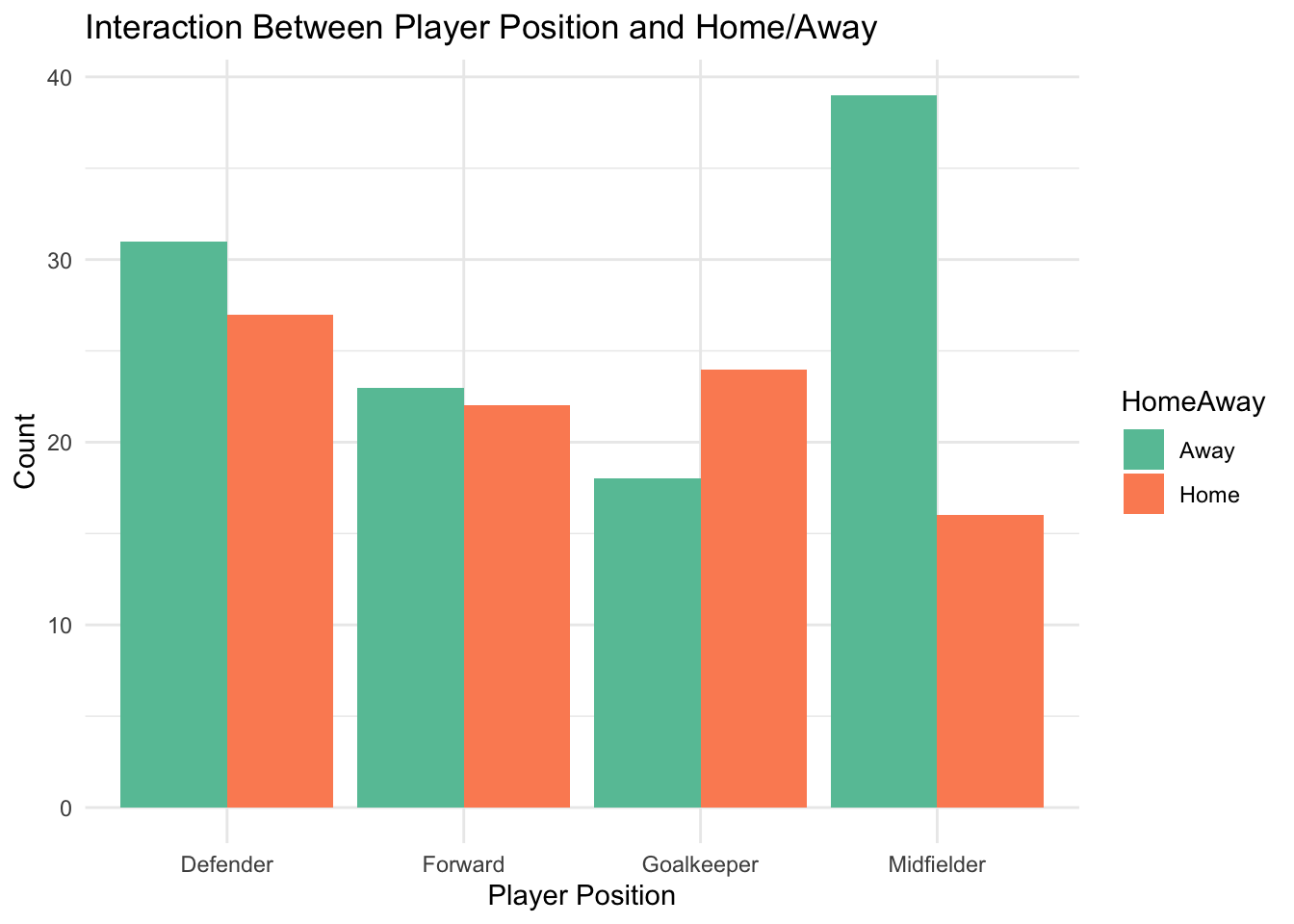
Interactions between categorical variables can provide important insights, but they also come with some challenges.
For instance, a player’s position (Forward, Midfielder) and home/away status may jointly affect match outcomes. Without accounting for these interactions, models may overlook important patterns.
To address interaction effects, we might use the following techniques:
Exploration: Visualise interactions (e.g., stacked bar plots) to identify relationships.
Feature Engineering: Create new categorical variables that specifically represent these interactions, such as “Forward-Home” or “Midfielder-Away.”
Regularisation: Use regularisation techniques (e.g., Ridge, Lasso) to prevent overfitting when including many interaction terms.
Sparse data refers to categories with few observations. Sparse categories can create ‘noise’ in the dataset and make model training unstable.
To address sparse data, we can use the following techniques:
Category reduction: Merge sparse categories into larger groups based on logical or statistical similarities.
Weight of Evidence (WoE): Replace sparse categories with a numeric measure of their predictive power, such as the log odds of a specific outcome.
Target encoding: Replace sparse categories with the mean value of the target variable for that category.
As I mentioned above, categorical data is central to many analytic processes in sport. For example, this form of data is crucial in:
Predicting match outcomes (e.g., Win, Loss, Draw), categorical variables such as team names, home/away status, weather conditions, and player formations play an important role.
Understanding the impact of different player roles (e.g., Forward, Midfielder) on match statistics can be useful for evaluating performance.
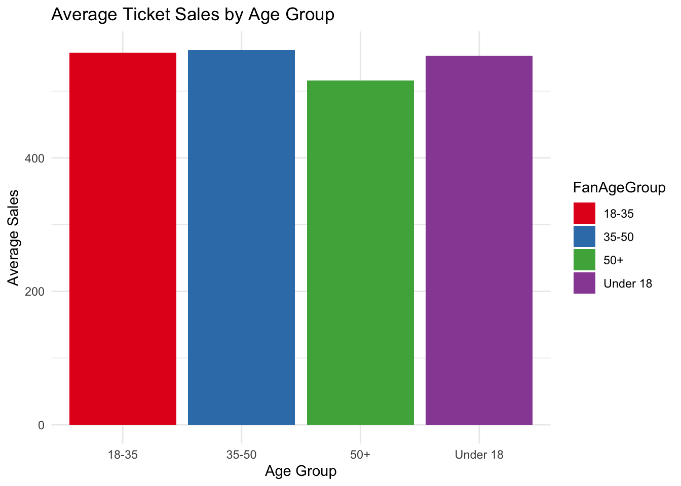
Understanding fan behaviour and engagement
R can handle categorical data through its range of libraries and functions. Some examples are given below.
R offers versatile tools for encoding and pre-processing categorical variables:
Factor Variables: R treats categorical data as factors, which can be nominal (unordered) or ordinal (ordered).
One-Hot Encoding: Libraries like caret and recipes facilitate one-hot encoding.
Handling Missing Data: Functions like ifelse() and mutate() can replace missing categories with meaningful substitutes.
Several R functions allow us to analyse categorical data directly:
Logistic Regression: We can use the glm() function to model binary outcomes, with categorical predictors included as factors.
Chi-Square Tests: We can perform independence tests using chisq.test() for contingency tables.
Measures of Association: We can libraries like DescTools for Cramer’s V and Phi coefficients.
Visualising categorical data is essential for exploring patterns and relationships. R’s ggplot2 package is great for creating:
Bar plots for category frequencies. Grouped or stacked bar charts for relationships between categories.
Mosaic plots for contingency tables.
Call:
glm(formula = WinBinary ~ PlayerPosition + HomeAway, family = "binomial",
    data = sports_data)

Coefficients:
                         Estimate Std. Error z value Pr(>|z|)
(Intercept)               0.02051    0.29767   0.069    0.945
PlayerPositionForward    -0.55083    0.41286  -1.334    0.182
PlayerPositionGoalkeeper -0.11407    0.41065  -0.278    0.781
PlayerPositionMidfielder -0.25319    0.38460  -0.658    0.510
HomeAwayHome             -0.34313    0.29872  -1.149    0.251

(Dispersion parameter for binomial family taken to be 1)

    Null deviance: 271.45  on 199  degrees of freedom
Residual deviance: 268.22  on 195  degrees of freedom
AIC: 278.22

Number of Fisher Scoring iterations: 4
    Pearson's Chi-squared test

data:  contingency_table
X-squared = 5.4072, df = 6, p-value = 0.4927
[1] 0.1162666